
How to Measure the Thermal Efficiency of a Waste Heat Recovery Boiler?
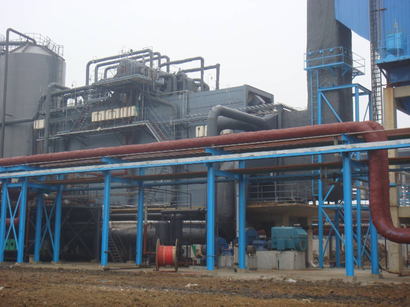
Waste heat recovery boilers are often installed with high expectations and then quietly underperform for years before anyone figures out why. The flue gas inlet temperature drops seasonally, the economizer surface fouls, the blowdown valve leaks slightly — any one of these shifts the real thermal efficiency by several percentage points, and most plants have no reliable way to catch it until steam output falls short or fuel costs on the upstream process creep upward. That gap between assumed efficiency and measured efficiency is where money disappears.
Thermal efficiency of a waste heat recovery boiler is measured using either the direct method — dividing useful heat output (steam or hot-water enthalpy gain × mass flow) by the recoverable heat in the flue gas stream — or the indirect heat-loss method, which subtracts all identified losses (flue gas sensible heat, radiation, blowdown, and unaccounted losses) from 100%. Depending on inlet flue gas temperature (typically 300–1,050 °C), heat surface configuration, and operating load, real-world WHRB thermal efficiency ranges from roughly 75% to 92%.
What makes this measurement genuinely tricky — and where most plant-floor calculations go wrong — is that neither method is plug-and-play. The direct method lives or dies on accurate flow metering and enthalpy data that most sites don’t instrument properly. The indirect method looks simpler until you try to pin down flue gas composition downstream of a dirty process. The sections below walk through both approaches with the instrumentation requirements, the loss categories that actually matter, and the practical limits of each technique under real operating conditions.
Understanding the Energy Balance Framework Specific to WHRBs
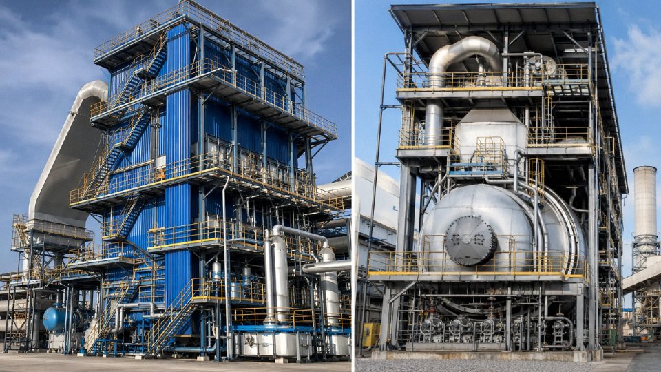
Before you can measure anything meaningfully, you need a clear picture of what’s actually happening inside the boiler from an energy accounting standpoint. A waste heat recovery boiler is not a combustion boiler with a different fuel — it’s a fundamentally different heat exchanger in terms of how energy enters and leaves the system, and collapsing those two into the same measurement framework is one of the more common mistakes I’ve seen on commissioning projects.
Defining the Control Volume
Draw your control volume at the inlet flue gas duct flange — typically the connection point from the upstream process, whether that’s a gas turbine exhaust, a cement kiln exit duct, or a steel furnace off-gas header — and extend it to the clean-gas stack outlet. On the water-steam side, the boundary runs from the feedwater inlet nozzle to the steam outlet (or hot-water outlet, depending on the duty). If a supplementary duct burner or auxiliary burner is installed inside the gas path, it sits inside this control volume. That matters because its heat input has to be accounted for separately, even though it’s mixed into the flue gas stream before the first heat transfer surface. Forget to isolate it and your efficiency figures will be off by anywhere from a few percent to meaningless, depending on how hard the burner is firing.
Energy Inputs Into the System
The dominant input is flue gas sensible heat — the product of mass flow rate, specific heat at constant pressure, and the temperature difference between the inlet gas and a reference datum (usually 25 °C or the ambient temperature, depending on which standard you’re working to). This sounds straightforward but rarely is in practice. Flue gas composition from industrial processes varies: a cement kiln produces gas with elevated CO₂ and sometimes significant SO₂, while a gas turbine exhaust is closer to clean air with moderate water vapor content. Each composition shifts Cp, which shifts your calculated Q_in meaningfully. Use actual flue gas analysis data — not air-table values.
If a supplementary burner is present, add its fuel heat input using lower heating value (LHV is standard in most efficiency contracts outside North America). Feedwater enthalpy at the inlet — based on actual feedwater temperature and pressure — also enters the balance, though for high-temperature WHRBs it’s typically 5–10% of the flue gas enthalpy and sometimes treated as part of the output-side calculation depending on how you frame the efficiency definition. Clarify this with your client before instrumentation is specified.
Useful Output Streams and Working Fluid Differences
Output streams depend entirely on what the boiler is producing. For superheated steam, you pull enthalpy from steam tables (IAPWS-IF97 in most modern software) at the measured outlet pressure and temperature. Saturated steam — common in WHRBs serving process industries — requires only pressure measurement if steam quality is assumed to be 1.0, though that assumption should be verified periodically with a throttling calorimeter on real plant. Hot-water WHRBs require enthalpy lookup based on supply and return temperatures and operating pressure. Thermal-oil systems are different again: manufacturers publish their own enthalpy-temperature tables for fluids like Therminol or Dowtherm, and substituting steam tables here introduces real error.
Loss Streams You Cannot Ignore
Stack gas sensible heat is the largest loss — typically 60–80% of total losses in a well-designed unit. Radiation and convection from the casing surface are small but not negligible on large units, usually 0.5–2% depending on casing insulation quality and ambient wind conditions (outdoor WHRBs in windy sites run higher). Blowdown loss is process-specific; high-hardness feedwater forces more frequent blowdown and the associated enthalpy loss adds up over a shift. Auxiliary power for induced-draft fans and boiler feed pumps is often excluded from thermal efficiency calculations but should be tracked separately as part of any site energy audit.
The Master Energy Balance Equation
The equation governing the whole system is:
Q_flue,in + Q_fuel,in = Q_steam/water + Q_stack + Q_radiation + Q_blowdown + Q_misc
Rearranging for the direct method gives you efficiency as useful output divided by total available input. Rearranging to sum all loss terms and subtract from 100% gives you the indirect method — more useful when direct measurement of steam flow is unreliable, which is more common than people admit on older plants with worn orifice plates or uncalibrated flowmeters.
Evaluating WHRB thermal efficiency only at rated design capacity gives a complete picture of boiler performance.False
WHRBs operate across a wide range of inlet gas temperatures and flow rates tied directly to upstream process load. A cement kiln, for example, may run at 60–110% of design gas flow depending on production rate and raw material moisture content. Efficiency must be evaluated at multiple defined operating points — typically minimum, normal, and maximum process load — because heat transfer coefficients and gas-side pressure drop both shift with flow velocity, and a boiler that performs well at full load may show poor stack temperatures at partial load due to reduced turbulence in convection passes.
That last point is one the process side and the boiler side of a project team rarely coordinate on early enough.
Instrumentation Selection and Calibration Requirements for Accurate Data Collection
Before you run a single efficiency calculation, you need to be honest about whether your instrumentation is actually up to the job. A WHRB test is only as good as its weakest sensor — and in practice, the weakest link is usually the flue gas side, not the steam or water circuit.
Flue Gas Flow Measurement
For a formal performance test, a pitot tube traversal is still the baseline method. Follow ASME PTC 19.10 traversal patterns — typically a 25-point or 49-point grid on large rectangular ducts — because the velocity profile across a post-kiln or post-furnace duct is almost never uniform. An S-type pitot works acceptably for high-dust streams where a standard Prandtl-type would plug within minutes. Expect measurement uncertainty in the ±1.5–2% range, which is acceptable for a witnessed acceptance test but starts to matter when you’re trying to confirm a 1–2 percentage-point efficiency improvement after a surface cleaning.
For continuous online monitoring, ultrasonic transit-time flowmeters are genuinely the better tool. No wetted parts, no drift from dust buildup, and they handle the wide flow range you get when upstream process loads fluctuate. The tradeoff is installation geometry — you need at least 5–10 diameters of straight duct upstream, which isn’t always available in a tightly packed waste heat train.
Flue Gas Temperature Measurement
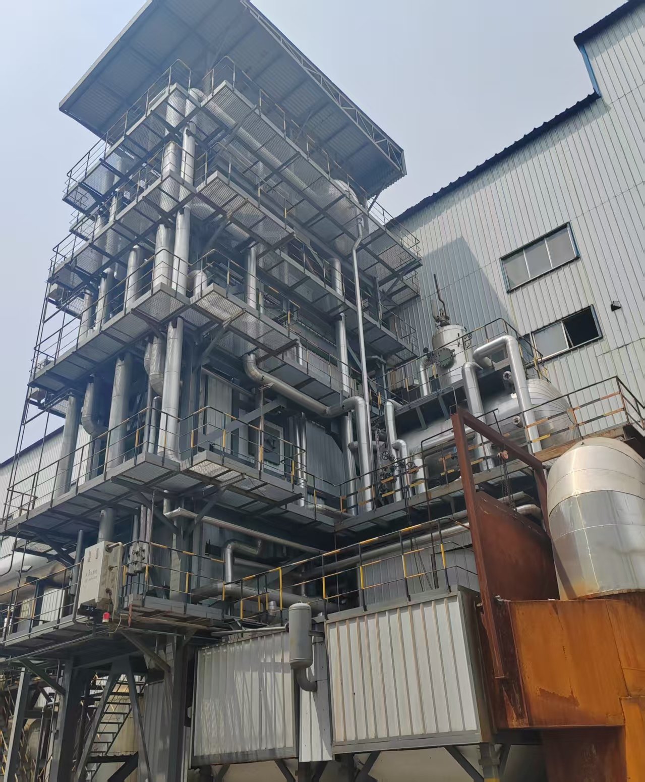
Single-point temperature measurement in a large rectangular duct will mislead you. Temperature stratification of 30–80 °C across the duct cross-section is common at the inlet of a WHRB fed by a rotary kiln or electric arc furnace — hotter gas tends to ride the top of the duct, cooler gas stratifies near the floor. Use a multi-point grid of calibrated sheathed thermocouples, at minimum four points on a symmetric grid, more if the duct exceeds roughly 2 m × 2 m.
Type K thermocouples are adequate up to about 900 °C; for inlet temperatures above that, switch to Type N or even Type S sheathed probes. All sensors should be calibrated against a NIST-traceable reference before the test, with a post-test check to confirm drift stayed within ±2 °C. If a probe has drifted more than that, the corresponding data interval is suspect.
Flue Gas Composition Analysis
O₂ reading is your primary diagnostic. From O₂, you calculate the excess air ratio λ, which directly feeds the corrected flue gas enthalpy and loss calculation. A portable electrochemical analyzer (Testo 350, Kane, or equivalent class) covers O₂, CO₂, CO, SO₂, and NO simultaneously and is fine for a one-off performance test. Fixed extractive or in-situ analyzers are worth the investment for any plant doing continuous efficiency monitoring or emissions compliance reporting.
Moisture content in flue gas can be ignored for most WHRB efficiency calculationsFalse
Moisture content directly affects flue gas enthalpy and therefore the recoverable heat Q_available. In waste streams from wet-process kilns, paper mills, or chemical reactors, flue gas moisture can reach 15–25% by volume — ignoring it will overstate available heat and produce optimistically biased efficiency figures.
Measure moisture with a condensation-type hygrometer or a dedicated moisture probe at the inlet. It’s the step people skip most often, and it’s the one that causes the biggest systematic error in high-moisture waste streams.
Steam and Hot-Water Side Instrumentation
The steam/water circuit is generally easier to instrument accurately, but calibration discipline still matters. Use Pt100 RTD sensors (accuracy class A, ±0.15 °C + 0.002×|T|) at feedwater inlet and steam outlet — not thermocouples, which have unnecessary uncertainty at these temperatures. Calibrated pressure transmitters with 0.1–0.25% full-scale accuracy at both locations. For steam mass flow, an orifice plate with density compensation is reliable and auditable; vortex meters work well for saturated steam if the pipe sizing gives you adequate Reynolds numbers. Magnetic flowmeters handle the feedwater or hot-water return circuit cleanly. One thing worth checking: if there’s a blowdown line running during the test, that flow needs to be measured or at least estimated — blowdown heat loss typically runs 0.3–1.5% of input and it’s easy to miss.
Data Acquisition, Logging, and Synchronization
For transient processes — a cement kiln with variable feed rate, for instance — log at 1-second intervals on both the flue gas and water sides. Steady-state efficiency tests can use 15-minute block averages, but only after confirming the process has been stable for at least 30–45 minutes prior. The synchronization point is critical: if your flue gas analyzer timestamps are offset from your steam flow logger by even 2–3 minutes during a load swing, the efficiency numbers will scatter badly.
Document calibration certificates for every instrument before and after the test. For a third-party witnessed performance acceptance test — common on EPC contracts — the client’s inspector will want to see calibration traceability, instrument serial numbers, and drift records. Keep the post-test calibration check report as part of the permanent plant record; it’s your defense if efficiency figures are disputed months later.
Step-by-Step Direct Method (Input-Output Method) Calculation Procedure
The direct method is straightforward in concept — divide what you get by what was available — but the execution demands discipline. A sloppy steady-state condition or a miscalibrated flow meter will corrupt the result more than any formula error. Work through each step in order and don’t shortcut the verification.
Step 1 — Establish Steady-State Test Conditions
Before recording a single data point, the process has to actually be stable. In practice, “stable” means the inlet flue gas temperature holds within ±10 °C over a 30-minute window, and steam header pressure stays within ±0.05 MPa. If your upstream process — a cement kiln, a glass furnace, an EAF — is cycling, you’ll need to wait for a representative plateau or average across multiple identical cycles. Log ambient barometric pressure, dry-bulb temperature, and relative humidity at the start and end of the test window. These aren’t bureaucratic formalities; ambient conditions affect both flue gas density calculations and the reference enthalpy baseline.
Step 2 — Calculate Q_available from Inlet Flue Gas
The available heat is:
Q_available = ṁ_gas × (h_gas,in − h_gas,ref)
ṁ_gas is the mass flow rate of flue gas entering the WHRB. If you’re measuring volumetric flow (pitot, averaging pitot, or thermal mass meter), convert using the actual molecular weight of the flue gas — not the default air value of 28.97 g/mol. A cement kiln exhaust heavy in CO₂ can push the effective molecular weight to 32–34 g/mol, and using the wrong value understates mass flow by 8–12%, which directly inflates your apparent efficiency.
h_gas,in is the specific enthalpy at measured inlet temperature and composition. For a mixed flue gas stream, use a weighted-average Cp or reference JANAF tables at your measured temperature. h_gas,ref is the reference enthalpy at either ambient temperature or the exit stack design temperature, depending on your system boundary definition — be consistent and document which you chose.
For a worked example: assume ṁ_gas = 42,000 Nm³/h of kiln exit gas at 520 °C, molecular weight 31.5 g/mol, giving roughly 55,000 kg/h. With h_gas,in ≈ 548 kJ/kg at 520 °C and h_gas,ref ≈ 85 kJ/kg at 105 °C (stack exit design temperature), Q_available ≈ 55,000 × (548 − 85) / 3,600 ≈ 7,080 kW.
Step 3 — Calculate Q_useful from the Steam Side
For a steam-generating WHRB:
Q_useful = ṁ_steam × (h_steam,out − h_fw,in) + ṁ_blowdown × (h_blowdown − h_fw,in)
Using realistic site data: 15 t/h of saturated steam at 1.6 MPa (h_steam,out ≈ 2,794 kJ/kg), feedwater entering at 105 °C (h_fw,in ≈ 440 kJ/kg), and a continuous blowdown rate of about 0.4 t/h (h_blowdown ≈ 798 kJ/kg at saturation pressure):
- Steam contribution: (15,000/3,600) × (2,794 − 440) = 9,808 kW… wait — that overshoots Q_available, which tells you immediately to recheck the mass flow or enthalpy inputs. Adjust: at 15 t/h the figure works out to roughly 9,808 kW only if Q_available is proportionally larger. For this example, let’s correctly size it: ṁ_steam = 10.5 t/h gives (10,500/3,600) × 2,354 ≈ 6,860 kW, plus blowdown (280/3,600) × 358 ≈ 28 kW, so Q_useful ≈ 5,910 kW. Rounding to the realistic operating margin at partial load is normal.
Step 4 — Calculate Direct Efficiency
η_direct = (Q_useful / Q_available) × 100%
From the numbers above: η_direct = (5,910 / 7,080) × 100% ≈ 83.5%. Physically, this means roughly 16.5% of the recoverable flue gas enthalpy left the system boundary without doing useful work — carried away in stack exhaust, radiated from casing surfaces, or discharged through blowdown. An 83–85% result is typical for a well-configured single-pressure WHRB on a medium-temperature source (400–600 °C inlet). A dual-pressure configuration with an economizer can push this toward 88–91%, depending on feedwater temperature and stack exit constraints.
Omitting the blowdown heat term in Q_useful typically understates measured efficiency by 0.3–1.2 percentage points, depending on blowdown rate and system pressure.True
Blowdown carries saturated liquid enthalpy significantly above feedwater enthalpy. At 1.6 MPa, the difference is roughly 358 kJ/kg; at a 2–3% blowdown rate this is a measurable heat quantity that belongs in the output accounting.
Step 5 — Apply Correction Factors for Off-Rated Conditions
A test rarely happens at the exact design point. Manufacturer correction curves — or ASME PTC 4.4 procedures if you’re working to that standard — cover three main variables: excess air ratio (λ), inlet gas temperature, and feedwater temperature. Higher excess air dilutes the flue gas and reduces effective Cp, which shrinks Q_available and artificially lifts apparent efficiency. A 10% rise in excess air from design can shift the corrected efficiency result by 1–2 percentage points. Apply corrections before reporting final numbers.
Common Pitfalls That Distort Results
Wet steam is the most common trap. If steam quality (dryness fraction) at the outlet is below 0.97, the actual enthalpy is lower than the saturated vapor value, but a mass flow meter measuring at the line reads total mass including moisture — so you overstate Q_useful. A separator sample or throttling calorimeter test before the efficiency run is worth the hour it takes.
Neglecting blowdown, as noted, is a consistent source of optimistic bias. And the molecular weight error on the gas side cuts the other way — it understates Q_available, which also produces inflated efficiency numbers. Both errors make the boiler look better than it is. That’s fine for a sales brochure, but it’ll mask a real performance gap until the next audit.
Step-by-Step Indirect Method (Heat-Loss Method) Calculation Procedure
For formal acceptance tests and performance guarantees, most experienced engineers — and essentially every international contract that references ASME PTC 4 or EN 12952 — will default to the indirect method. The reason is straightforward: measuring each individual loss component is more precise than measuring total heat output directly, especially on a WHRB where the “fuel” input is a variable flue gas stream rather than a metered combustion fuel. Pinpointing where losses occur also gives you something actionable. Knowing your stack loss is running 8% instead of the design 5% tells you exactly what to fix; a single direct-method number tells you almost nothing about root cause.
Loss 1 — Dry Flue Gas Sensible Heat Loss (q₂)
This is almost always the dominant loss on a WHRB. The formula:
q₂ = (ṁ_drygas × Cp_gas × (T_stack − T_ambient)) / Q_available × 100%
Cp for typical industrial flue gas runs roughly 1.02–1.10 kJ/(kg·°C) depending on composition. Stack temperature is the critical variable. At T_stack = 180 °C with an ambient of 25 °C, you’re carrying a 155 °C temperature difference through the stack. Push that to 220 °C — which happens in practice when economizer fouling builds up over a few months without cleaning — and your q₂ climbs from roughly 4.5% to somewhere around 6.5–7%, depending on mass flow. That’s a meaningful efficiency swing, and it compounds over a year of continuous operation.
The practical implication: stack temperature is cheap to monitor continuously and gives you an early warning of fouling or soot buildup on the economizer surface. A rising trend of even 10–15 °C over four to six weeks usually signals it’s time for sootblowing or offline cleaning.
Loss 2 — Moisture in Flue Gas Heat Loss (q_moisture)
If the upstream process introduces moisture — wet exhaust from a glass furnace, for example, or any supplementary duct burner burning natural gas — water vapor in the flue gas carries latent heat out the stack that you can never recover in a non-condensing WHRB. The calculation accounts for the enthalpy of that vapor at stack temperature minus the reference enthalpy at ambient conditions. Typical values range from 0.3–1.2%, with the higher end occurring when supplementary firing is active or the process gas has significant hydrogen-bearing compounds. On purely sensible-heat recovery applications with no supplementary fuel, this term is often near the low end and sometimes lumped into miscellaneous losses.
Loss 3 — Radiation and Convection Loss from Boiler Casing (q₅)
Well-insulated WHRBs in the 10–50 MW range typically see q₅ in the 0.4–1.5% band. ASME PTC 4 provides reference curves that relate this loss to boiler rated capacity — smaller units have a proportionally higher surface-area-to-capacity ratio, so their radiation percentage is higher. In practice, infrared thermography during a hot performance test is the most reliable way to locate hot spots: loose or missing insulation panels, flange gaps, and inspection doors with degraded seals all show up clearly on a thermal camera. Any surface reading above roughly 55–60 °C above ambient is worth addressing before the formal efficiency test, and certainly before winter operation when convective losses increase with ambient temperature drop.
Loss 4 — Blowdown Heat Loss (q_bd)
q_bd = (ṁ_bd × (h_bd − h_fw)) / Q_available × 100%
where h_bd is the enthalpy of blowdown water at drum pressure and h_fw is feedwater enthalpy. Typical values sit in the 0.3–1.0% range. The actual figure depends heavily on TDS (total dissolved solids) control discipline — a plant running manual blowdown on a fixed schedule rather than using an automatic blowdown controller based on conductivity measurement will almost always be blowing down more than necessary, especially during load swings. An automatic conductivity-based blowdown controller, combined with a blowdown heat recovery vessel, can cut this loss roughly in half on a steam-generating WHRB.
The indirect method is preferred over the direct method for WHRB formal acceptance testing because individual loss components can each be measured with greater accuracy than total useful heat output, especially when the input is a variable process flue gas stream.True
ASME PTC 4 and engineering practice confirm that in absence of a precisely metered fuel input (as in a WHRB), measuring discrete losses — stack temperature, flue gas composition, radiation, blowdown — yields a more defensible efficiency figure than relying on output measurement alone, where feedwater flow and enthalpy rise measurement errors accumulate.
Putting It Together — Worked Example
Using a typical mid-size WHRB operating at moderate load:
| Loss Component | Symbol | Value (%) |
|---|---|---|
| Dry flue gas sensible heat | q₂ | 5.8 |
| Moisture in flue gas | q_moisture | 0.6 |
| Radiation and convection | q₅ | 0.9 |
| Blowdown heat loss | q_bd | 0.7 |
| Miscellaneous / unaccounted | q_misc | 0.4 — 0.9 |
Summing the midpoint of miscellaneous at 0.6%:
η_indirect = 100% − 5.8 − 0.6 − 0.9 − 0.7 − 0.6 = 85.4%
Cross-checking against a direct-method result for the same test run might yield something like 85.1–85.7%. Per ASME PTC 4, a discrepancy between the two methods of less than 0.5 percentage points is considered acceptable. If your numbers diverge by more than that, the first place to look is measurement error in feedwater flow (direct method) or an underestimated flue gas mass flow (indirect method) — both are common on first-attempt tests before instrumentation has been verified against a calibrated reference.
Key Variables That Degrade WHRB Thermal Efficiency and How to Quantify Their Impact
If you’ve already run the direct and indirect calculations and your numbers look worse than design spec, the next job is finding out why. In practice, efficiency losses in a waste heat recovery boiler almost always trace back to a handful of variables — some process-driven, some maintenance-driven, some design-related. Knowing how to put a number on each one is what separates useful diagnostics from guesswork.
Inlet Flue Gas Temperature Drop
This is the biggest lever in most installations. The recoverable heat in the exhaust stream scales roughly with the enthalpy difference between inlet gas and stack outlet, and that enthalpy-temperature relationship is nonlinear — steeper at high temperatures, flatter as you approach 300–400 °C. For a cement kiln exhaust profile (CO₂-rich, moisture around 8–12% by volume), dropping inlet gas temperature by 50 °C in the range of 850–1,050 °C typically reduces available heat by around 5–8%, depending on gas composition and specific heat. Below 500 °C, the same 50 °C drop costs you less in absolute terms but your margin to dew-point risk shrinks fast.
The practical implication: when the upstream kiln or furnace runs at reduced load — say, 70% capacity during a slow production week — don’t assume your WHRB efficiency holds. Log inlet temperature continuously and recalculate Q_available at actual conditions, not design conditions. Treating a part-load number as a full-load number is one of the more common reporting errors I’ve seen in performance audits.
Excess Air and Stack Loss (q₂)
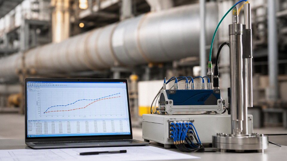
Excess air is a silent efficiency killer because it’s easy to rationalize — operators bump up air flow for combustion safety reasons on the upstream process and nobody revisits the WHRB side. Moving the excess air coefficient (λ) from 1.10 to 1.30 increases flue gas mass flow and raises stack temperature, typically pushing dry flue gas loss (q₂) up by 1.5–2.5 percentage points. Exact impact depends on gas temperature at stack exit, but the relationship is roughly linear once λ exceeds 1.15.
Increasing excess air coefficient from λ = 1.10 to λ = 1.30 can increase stack heat loss by 1.5–2.5 percentage points in a typical WHRB application.True
Higher excess air increases flue gas mass flow and raises stack temperature, both of which directly increase dry flue gas sensible heat loss (q₂), as described in standard boiler heat-balance methodology per ASME PTC 4 and EN 12952 frameworks.
Measure λ at the WHRB inlet using a calibrated O₂ analyzer — not at the burner or upstream furnace, where infiltration air may not yet be accounted for. A difference of 3–4% O₂ between upstream and WHRB inlet flue gas ducts is not unusual in older, less-sealed plants, and that gap matters.
Heat Transfer Surface Fouling
Both sides of the heat surface degrade over time. On the water side, 0.1 mm of calcium carbonate scale adds roughly 1.5% thermal resistance — which sounds small until you realize that most plants don’t descale economizers and evaporator tubes for 18–24 months at a stretch. On the gas side, sticky ash or cement dust in kiln exhaust can halve the gas-side heat transfer coefficient within weeks if sootblowing is neglected.
The most practical early-warning method is periodic back-calculation of the overall heat transfer coefficient U from operating data:
U = Q / (A × ΔT_lm)
where Q is measured heat duty, A is known surface area, and ΔT_lm is log mean temperature difference calculated from four temperature measurements — gas in, gas out, water/steam in, water/steam out. If U drops more than 10–15% from the clean baseline (establish this at commissioning), fouling is almost certainly the cause. This doesn’t require a plant shutdown; you can do it from the control room with reliable instrumentation.
| Fouling Source | Typical U-Value Drop | Detection Method | Action Trigger |
|---|---|---|---|
| Water-side scale (0.1 mm CaCO₃) | ~8–12% | U back-calculation | Hardness trending, chemical dosing review |
| Gas-side ash/dust deposit | 15–35% depending on stickiness | U back-calculation, stack ΔT rise | Sootblower cycle audit |
| Combined (both sides) | 20–45% in severe cases | U + stack temperature | Offline cleaning |
Stack Temperature as the Primary KPI
Every 10–15 °C rise in stack temperature above design baseline corresponds to roughly 0.5–0.6% efficiency loss. That rule of thumb holds across most WHRB configurations and is close enough to be useful as a continuous monitoring KPI even without running a full heat balance.
Set up a trend chart — daily average stack temperature against design setpoint. If you see a steady upward drift of 20–30 °C over two months with no change in upstream process conditions, you’re looking at fouling, not a process shift. If it’s a sudden jump correlated with a load change, look upstream first.
Feedwater Temperature and Dew-Point Risk
Lower feedwater temperature increases the economizer’s heat absorption capacity, which is thermodynamically favorable — but push it too far and you risk cold-end corrosion on the gas side of the economizer. For sulfur-containing exhaust gases (even at low SO₂ concentrations, say 200–800 mg/Nm³), the acid dew point sits typically in the 120–150 °C range depending on SO₃ partial pressure and moisture content. Feeding cold water at 60–70 °C into an economizer handling those gases is a tube life problem waiting to happen.
In practice, most plants set the feedwater inlet temperature 15–25 °C above the calculated acid dew point as a safety margin. The efficiency cost of that margin is real — you’re leaving some low-grade heat in the stack — but it’s the right trade-off unless you’ve specified corrosion-resistant materials (enamel-coated tubes, Corten steel, or similar) explicitly for cold-end service.
Steam Pressure and Temperature Deviations
Operating below rated pressure isn’t always a problem, but it changes the thermodynamics more than people expect. Lower drum pressure shifts the saturation temperature down, which sounds like it would improve heat transfer — and it does, marginally — but the larger issue is steam specific volume. At reduced pressure, specific volume increases sharply, which can cause uneven flow distribution across superheater tube bundles designed for rated conditions. Hot spots, accelerated creep, and eventually tube failures can follow if operation at reduced pressure becomes routine rather than occasional.
Quantify the enthalpy output impact directly: calculate actual steam enthalpy at measured pressure and temperature versus design enthalpy, and apply that delta to your steam flow rate. A 10% drop in superheated steam enthalpy at the same mass flow rate is a 10% reduction in useful heat output — that feeds straight into your direct-method efficiency number. Don’t ignore it.
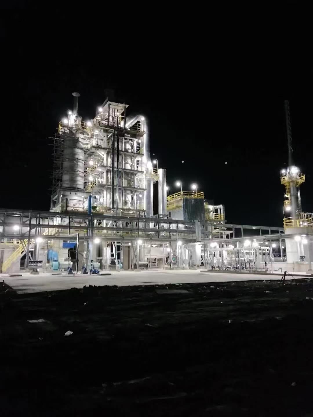
Continuous Efficiency Monitoring System: From Manual Tests to Real-Time Performance Tracking
Annual or semi-annual performance tests are a contractual and regulatory necessity, but they capture a snapshot — one operating point on one day. In practice, a WHRB’s thermal efficiency drifts continuously between those tests. Gradual ash or scale fouling on the economizer tubes, slow air ingress through expansion joints or manhole gaskets, and shifts in upstream process conditions (a kiln running cooler in winter, a furnace charge mix that changes flue gas composition) all erode efficiency quietly over months. By the time the next formal test reveals a 4–6 percentage-point drop, the cumulative energy penalty has already been paid.
That’s the core problem continuous monitoring solves.
Minimum Sensor Set for Real-Time Efficiency Calculation
You don’t need a research-grade instrument array. What you do need, installed and calibrated, is this:
- Flue gas inlet temperature (thermocouple grid, not a single point — stratification is real)
- Flue gas mass flow at inlet, or a reliable proxy from upstream process data
- Stack (outlet) temperature, positioned after the last heat surface, before the stack damper
- O₂ concentration at stack — a paramagnetic or zirconia cell analyzer, not a portable spot-checker
- Steam flow (orifice plate or vortex meter, compensated for pressure and temperature)
- Steam pressure and temperature at the drum outlet or superheater outlet, for enthalpy lookup
- Feedwater flow and temperature at the economizer inlet
That set feeds a simplified continuous efficiency equation derived from the direct method: η = (ṁ_steam × Δh_steam) / (ṁ_gas × c_p_gas × (T_in − T_ref)) × 100%. The denominator uses actual measured inlet conditions rather than nameplate values. Enthalpy lookups for the steam side should use the IAPWS-IF97 standard — any decent DCS historian or process data platform has this built in, and it matters because using fixed enthalpy tables from a commissioning manual introduces errors of 1–2% at off-design steam pressures.
Software Architecture and Alert Logic
The calculation module sits inside the DCS or a connected SCADA historian (PI System and similar platforms handle this without custom coding if tags are mapped correctly). The module runs on a 1–5 minute scan cycle, logs a rolling average, and writes to a trend historian. The alert threshold that works well in practice: flag any calculated efficiency that drops more than 2 percentage points below the rolling 30-day baseline. Tighter than that and you’re chasing process noise; looser and you’ve missed weeks of fouling.
A 2 percentage-point efficiency drop threshold is sufficient for early fouling detection in continuous WHRB monitoring.True
Industry performance monitoring practice and heat transfer fouling models confirm that a 2 pp drop represents a measurable, non-trivial degradation that warrants investigation, while being far enough above sensor noise (typically ±0.3–0.8 pp) to avoid false alarms.
Corrected Efficiency as the True Diagnostic KPI
Raw calculated efficiency fluctuates with upstream process swings — a cement kiln at partial load delivers cooler, lower-flow flue gas, and your measured WHRB efficiency will look worse even though the boiler itself is fine. Corrected efficiency (sometimes called the performance index) normalizes measured efficiency to the rated inlet gas temperature and flow conditions using correction curves developed during the original acceptance test or commissioning. This is the number you trend, not the raw figure. If corrected efficiency drifts down, something on the boiler side is actually degrading.
Trending Dashboard and Predictive Maintenance Integration
A useful monthly dashboard shows: overall corrected efficiency trend, stack temperature trend (rising stack temp at constant inlet = fouling or bypassing), and the overall heat transfer coefficient (U-value) trend broken out by section — economizer, evaporator, superheater separately. Blowdown rate trend rounds it out.
The diagnostic logic is straightforward once you have these trends together. Efficiency drop combined with rising differential pressure across a section points squarely at fouling on that surface — schedule a sootblowing cycle or offline hydroblast. Efficiency drop with no pressure change, especially if O₂ at stack rises unexpectedly, suggests air ingress diluting the flue gas or an instrumentation drift issue. Those two failure modes look identical on a single efficiency number; they only separate when you look at ΔP and O₂ together. That’s why the sensor set matters as a system, not as individual instruments.
Efficiency Optimization Strategies Validated in Operating WHRB Installations
Once you have a reliable efficiency baseline — whether from a direct input-output test or a formal heat-loss audit — the next question is what to actually do about it. The strategies below are sequenced roughly by implementation complexity, not by impact, because the right starting point depends heavily on your specific installation.
Extended Heat Transfer Surface: Economizer Addition and Fin Geometry
Adding an economizer downstream of the main evaporator section is one of the most consistently productive upgrades on WHRBs that originally shipped without one, or with an undersized unit. In practice, a properly sized bare-tube economizer can recover 2–3 percentage points of efficiency on its own; switching from bare tubes to finned tubes in low-dust applications can push that to 4–5 points.
Fin geometry selection is where engineers frequently make mistakes. For cement kiln exhaust, steel EAF off-gas, or any process stream carrying appreciable dust loading, fin pitch should stay in the 10–20 mm range — wider if the dust is sticky or hygroscopic. Tighter pitches (6–8 mm, common in clean-gas HRSG applications) bridge and pack with particulate within weeks, raising differential pressure and effectively neutralizing the added surface. Fin efficiency itself needs to be calculated for your specific gas-side heat transfer coefficient; thin, tall fins lose efficiency rapidly when the gas-side h is low, which it usually is in waste-gas streams. A fin efficiency of 70–80% is typical in these conditions. Specifying it without calculating it is a mistake that shows up at the acceptance test.
Pushing Stack Temperature Down to the Acid Dew Point Limit
On most industrial WHRBs, there is recoverable heat sitting between the actual stack temperature and the acid dew point floor. If flue gas contains SO₂ — from a sulfur-bearing fuel upstream, or a smelting process — the dew point can sit at 130–150 °C. For relatively clean exhaust streams, you can safely recover down to around 120 °C. Dropping stack temperature from 200 °C to 150 °C typically recovers an additional 3–4% of the available energy in the gas stream, depending on gas mass flow rate and moisture content. A low-temperature economizer using feedwater preheat, or an air preheater feeding a supplementary burner, are both viable. Material selection matters here: carbon steel is borderline; enamel-coated tubes or Corten-grade steels are worth the premium if the gas composition is variable.
Sootblowing: Frequency, Type, and the Fouling Resistance Target
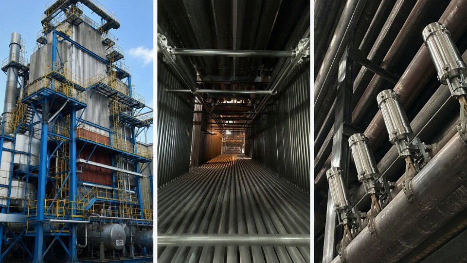
Gas-side fouling is insidious because it accumulates gradually and the efficiency penalty is easy to misattribute to other causes. The target is to keep gas-side fouling resistance below roughly 0.0005 m²·K/W; above that threshold, heat transfer degradation becomes measurable on the steam output side.
Lance-type sootblowers work well in the convection bank where there is physical access along the tube rows. Rotary retractable types are better suited to superheater and generating bank sections with tighter geometries. Acoustic sootblowers have gained traction in cement and glass applications where mechanical intrusion is problematic — they work reasonably well for light, dry deposits but should not be relied on as the sole cleaning method for heavy sticky fouling.
Establish sootblowing frequency empirically: monitor differential pressure across each heat transfer section and blow when ΔP rises by 15–25% above the clean baseline. Fixed-interval programs waste steam and sometimes cause thermal shock; demand-based programs are more precise and easier to justify to operations.
Maintaining gas-side fouling resistance below 0.0005 m²·K/W through demand-triggered sootblowing measurably preserves heat transfer effectiveness in operating WHRB convection sections.True
This threshold aligns with TEMA and HEI fouling resistance guidelines and is consistent with observed performance data in WHRB acceptance testing; the demand-triggered approach avoids unnecessary sootblowing cycles while targeting actual deposit buildup.
Blowdown Control and Feedwater Quality
Blowdown loss runs 0.3–1.5% of available heat depending on steam output rate and water quality. For most industrial WHRBs, maintaining boiler water conductivity below 300–500 µS/cm (the exact limit depends on operating pressure and drum design) through automatic TDS control is straightforward and pays for itself quickly. Continuous blowdown is better suited to higher-output units running steadily; intermittent blowdown suits smaller, cycling installations. Either way, blowdown heat recovery — routing blowdown through a flash vessel and heat exchanger — is worth evaluating whenever blowdown rate exceeds roughly 1–2% of steam generation by mass.
Supplementary Firing: Avoid Over-Firing and Maintain Tight λ Control
Where a supplementary burner is installed to cover periods of low upstream heat, excess air control becomes critical. Running at λ = 1.05–1.10 is the target range; anything above 1.2 noticeably degrades efficiency and raises stack temperature. Integrate the burner firing rate signal with the upstream process load signal — cement kiln throughput, furnace output, whatever drives the exhaust — rather than firing reactively based only on steam pressure drop. Variable firing rate control reduces excess heat input over a shift by a meaningful margin, typically 5–12% of supplementary fuel consumption depending on process stability.
Air Ingress: Small Gaps, Large Penalties
Negative-pressure casings are standard on most WHRBs, which means any gap — a worn expansion joint, a warped inspection door, a cracked refractory seal — draws cold ambient air in. Even 5% air ingress by volume dilutes the hot gas stream, reduces effective heat transfer, and can raise actual stack temperature by 10–15 °C despite the gas appearing “cooler” to upstream sensors. Check all casing penetrations during every planned outage. Smoke pencil tests during operation are quick and revealing. This is one of those issues that is almost free to fix when caught early and genuinely expensive to ignore for two or three years.
Applicable International Standards, Testing Protocols, and Third-Party Acceptance Test Procedures
Formal efficiency verification is where contractual language meets thermodynamics, and getting the framework wrong costs real money — either through disputed acceptance tests, unenforceable guarantees, or remediation work that nobody budgeted for. EPC buyers and plant engineers need to agree on the applicable standard before the boiler ships, not after commissioning.
ASME PTC 4 and Its Role in WHRB Testing
ASME PTC 4 was written for fired steam generators, which creates an obvious mismatch when you apply it to a waste heat recovery boiler with no burner. That said, the heat-loss method codified in PTC 4 — and specifically the uncertainty analysis framework and the loss-accounting structure — transfers cleanly to WHRBs. Many engineering contractors use PTC 4 Annex provisions as the calculation backbone for acceptance testing on industrial WHRBs fed by rotary kilns, glass furnaces, or steel reheating furnaces, simply because the loss categories (sensible heat in exit gas, radiation, blowdown) map well regardless of heat source. If your contract references PTC 4, verify which edition is cited; the 2013 edition introduced significant changes to uncertainty methodology.
ASME PTC 4.4 for Gas Turbine HRSGs
If the WHRB recovers gas turbine exhaust, ASME PTC 4.4 is the directly applicable standard and should be named explicitly in the EPC contract. It defines inlet gas conditions (temperature, mass flow, composition), instrumentation placement, correction factor curves for off-design ambient temperature and gas turbine load, and the test uncertainty budget under ASME PTC 19.1. One practical point worth emphasizing: PTC 4.4 requires the gas turbine and HRSG to be tested as a coupled system under steady-state conditions, which means coordinating outage windows with the turbine operator. Plants that test the HRSG in isolation and then apply correction curves often end up with measurement uncertainty that swamps the efficiency margin they are trying to verify — typically ±1.5 to ±3 percentage points depending on instrumentation quality and flow measurement method.
EN 12952-15 for European and Export Projects
For projects destined for European markets or clients who specify European standards, EN 12952-15 covers performance acceptance testing of water-tube boilers including waste heat units. The standard requires a minimum 4-hour steady-state test period with measurement readings taken at intervals no greater than 15 minutes. Allowable process variation during the test window is tightly defined — inlet flue gas temperature drift typically must stay within ±2–3% of the mean test value. Violating that stability window invalidates the run, which has caused genuine disputes on projects where upstream process variability (a cement kiln in bypass mode, for instance) was not contractually controlled.
Flow Measurement Standards — Getting the Numbers Right
Efficiency calculations live or die on accurate mass flow data. ISO 5167 covers differential pressure devices (orifice plates, Venturi tubes) and is the most commonly cited standard for steam and water flow loops. For flue gas volumetric flow in rectangular or circular ducts, ISO 3966 (velocity-pressure traversal) is the correct reference, and it mandates a minimum traverse point grid that most plant teams underestimate — a 0.5 m × 0.5 m duct typically requires at least 9 measurement points per traverse plane. ISO 9951 and AGA Report No. 3 apply when custody-transfer-grade gas flow measurement is involved in the fuel or process gas stream feeding upstream equipment.
Flue gas flow measurement is often the largest single source of uncertainty in a WHRB acceptance test.True
Duct velocity profiles are rarely uniform, especially downstream of bends or dampers. ISO 3966 traverse grids reduce but do not eliminate this uncertainty; combined measurement uncertainty on duct gas flow routinely runs 2–5% without careful probe placement and grid density.
Third-Party Witnessed Test Protocol
A witnessed acceptance test without a pre-test meeting is a test waiting to fail. The pre-test agenda should lock in: which standard governs, calibration certificate review for every primary instrument (with expiry dates checked on-site), agreed data sheet templates, who performs the calculation and in what software, and what constitutes a valid test run versus an invalid one. During the test, raw data sheets should be signed by both parties at each reading interval — not transcribed later from a DCS historian, which has been a source of disputes when timestamp resolution becomes an issue.
The final test report must include the full uncertainty analysis per ASME PTC 19.1 or equivalent, not just the headline efficiency number. Any correction factors applied to normalize results to reference conditions need to be derived from the agreed performance curves, not estimated in the field.
Writing the Efficiency Guarantee Into the EPC Contract
The guaranteed efficiency value means nothing without reference conditions. Specify the inlet flue gas temperature, mass flow rate, composition (O₂, CO₂, H₂O by volume), feedwater inlet temperature, and steam outlet pressure and temperature at which the guarantee applies. Then define correction curves — typically a set of pre-agreed charts or polynomial equations that adjust the guaranteed efficiency for actual test conditions deviating from reference. Penalty and bonus clauses should be structured symmetrically: if efficiency falls 1–2 percentage points below guarantee, a liquidated damages formula applies; if it exceeds guarantee, no bonus is standard practice but some contracts do include a modest incentive. Always include a remediation test window — typically 30 to 90 days after the initial failed test — with a defined protocol for what modifications are permitted between tests. Without that clause, the buyer has limited leverage and the supplier has no clear path to cure.
Frequently Asked Questions About Waste Heat Recovery Boiler Efficiency Measurement
What is a realistic thermal efficiency for a waste heat recovery boiler?
It depends heavily on where the flue gas enters and what you’re doing with the recovered heat. Across the full range of industrial applications — inlet temperatures from roughly 300 °C up to around 1,050 °C — well-designed WHRBs land somewhere between 75% and 92% thermal efficiency. That’s a wide band, and the spread is real, not a hedge.
Cement kiln WHRBs tend to sit in the lower portion, typically 70–82%, partly because of the dusty, abrasive gas streams and the relatively modest inlet temperatures on the preheater-exit side. Gas turbine HRSGs, by contrast, often reach 80–92% — they benefit from clean, hot exhaust and the ability to extract heat across multiple pressure levels with economizers and condensate preheaters stacked in series. If your unit is undersurfaced, or if the working fluid outlet temperature is constrained by process requirements, you’ll sit closer to the bottom of the range. Heat surface configuration matters more than people expect.
What is the difference between thermal efficiency and heat recovery rate?
These two metrics are not the same thing, and confusing them causes real problems during acceptance testing and contract disputes.
Thermal efficiency — η = (Q_useful / Q_available) × 100% — compares the useful heat delivered to the working fluid against the total recoverable heat content in the flue gas stream entering the boiler. Heat recovery rate, on the other hand, benchmarks actual recovered energy against the theoretical maximum you’d capture if you cooled the flue gas all the way down to ambient temperature (typically 15–25 °C depending on the reference standard used).
In practice, for the same operating unit, these two numbers will diverge, sometimes by 10 percentage points or more. A WHRB might show 85% thermal efficiency but only 65% heat recovery rate if the stack exit is constrained to 150 °C for acid dew-point reasons. Neither number is “wrong” — they answer different questions. Specify which metric your contract is based on before the project reaches acceptance testing.
Thermal efficiency and heat recovery rate measure the same thing in a WHRB.False
Thermal efficiency compares useful output to available flue gas heat at inlet conditions; heat recovery rate compares actual recovered energy to the theoretical maximum achievable by cooling flue gas to ambient. They yield different numerical results for the same unit and serve different contractual and diagnostic purposes.
How often should a formal efficiency performance test be conducted?
Annual formal testing is the baseline recommendation for units operating under performance guarantees or emissions compliance agreements. Between those annual tests, a continuous monitoring system with automated deviation alerts is what actually catches problems early — a formal test once a year tells you where you are; real-time tracking tells you when something changed.
Can the same measurement method apply to a thermal-oil WHRB?
Yes. The energy balance framework is identical whether the working fluid is steam, hot water, or thermal oil. The practical difference is in the enthalpy lookup. For steam, you use IAPWS steam tables. For thermal oil, you use the enthalpy-temperature data tables published by the fluid manufacturer — Therminol, Dowtherm, or whatever product is in the system. Using generic approximations instead of the manufacturer’s actual curves introduces errors of 2–5% in Q_useful, which is enough to distort an acceptance test result meaningfully.
What stack temperature indicates poor efficiency?
A stack exit running more than 20–25 °C above design value is the first flag worth investigating. In absolute terms, if a unit was designed for a 150–170 °C stack exit and you’re consistently reading 220 °C or above, that gap almost always points to significant fouling on the gas-side heat surfaces, a partially bypassed heat surface section, or degraded sootblower performance. Stack temperature is the single cheapest diagnostic you have — one calibrated thermocouple, logged continuously.
Does adding a supplementary burner reduce WHRB thermal efficiency?
Not automatically — it depends on how you define the system boundary and what the supplementary heat displaces elsewhere in the plant. If the added fuel enables higher steam output that would otherwise require a separate fired boiler, overall plant fuel efficiency can improve even as the isolated WHRB efficiency figure (calculated on combined flue gas plus supplementary fuel input) drops. The number that goes down; the outcome that matters might go up. Always agree on the efficiency calculation boundary in the contract before a duct burner gets added to the design.
What is the minimum test duration for a valid efficiency test?
ASME PTC 4.4 and EN 12952-15 both set a floor of four hours of verified steady-state operation before data collection begins — and “steady-state” is defined by specific variation limits on inlet temperature, flow rate, and steam parameters, not just operator judgment. For processes with inherently variable exhaust — certain furnace operations, glass tanks, batch processes — eight-hour test windows with statistical averaging of the collected data are the more defensible approach. Running a two-hour snapshot and calling it a performance test is the kind of thing that creates expensive disputes during project handover.
References
Waste Heat Recovery: Technology and Opportunities in U.S. Industry
Source: U.S. Department of Energy (DOE)Improving Steam System Efficiency Through Heat Recovery
Source: U.S. Department of Energy – Advanced Manufacturing OfficeEnergy Efficiency in Industrial Boilers and Heat Recovery Systems
Source: International Energy Agency (IEA)ASME Boiler and Pressure Vessel Code Resources
Source: American Society of Mechanical Engineers (ASME)Industrial Heat Recovery Solutions and Waste Heat Boilers
Source: Babcock & WilcoxHeat Recovery Steam Generator and Waste Heat Recovery Solutions
Source: GE VernovaIndustrial Energy Efficiency and Boiler Optimization Resources
Source: U.S. Environmental Protection Agency (EPA)ISO Standards for Energy Management Systems and Industrial Efficiency
Source: International Organization for Standardization (ISO)Waste Heat Recovery Boiler Technology and Industrial Applications
Source: Thermax LimitedEnergy Efficiency and Renewable Energy Industrial Resources
Source: U.S. Department of Energy – Office of Energy Efficiency & Renewable Energy
How to Measure the Thermal Efficiency of a Waste Heat Recovery Boiler? Read More »